How I Built a Software Render Engine from Scratch

Heads Up: This ar­ti­cle is a re­pub­lished (with some tweaks on spelling, gram­mar and lay­out) ver­sion of an ar­ti­cle I wrote in my se­nior year of high school for my Linear Algebra class. As such, the pub­lish date is not quite cor­rect.

Computers are fan­tas­tic at pro­cess­ing, pro­duc­ing, and con­sum­ing data. But I’ve of­ten found that the most dif­fi­cult part of the pipeline is rep­re­sent­ing the data to a user. This can of­ten take the form of bar charts or scat­ter plots, but there are sit­u­a­tions where they just don’t fit the bill.

3D graph­ics en­able de­vel­op­ers to cre­ate in­ter­ac­tive pro­grams that ap­pear most sim­i­lar to the nat­ural world. By pre­sent­ing a three-di­men­sional space, the bar­ri­ers for en­try drop. I wanted to learn more about how this worked.

Inspiration

For a long time, I’ve been told that the most preva­lent ap­pli­ca­tion of lin­ear al­ge­bra was com­puter graph­ics. Be­fore I even be­gan my study on lin­ear al­ge­bra, I knew I wanted to get into soft­ware ren­der­ing.

One of the big road­blocks was the amount of tech­ni­cal know-how I thought it re­quired. You see, most 3D pro­grams do all the num­ber-crunch­ing on the spe­cially de­signed graph­ics pro­cess­ing unit that is read­ily avail­able on most mod­ern com­put­ers. From my pre­vi­ous at­tempts to use GPUs, I knew set­ting up the pipeline is quite in­volved. If I went that route again, I know I would likely spend most of my time deal­ing with ven­dor-spe­cific APIs.

Since I wanted to fo­cus on the math, I post­poned the pro­ject. That is, un­til it oc­curred to me that I could sim­ply not use the GPU. I know it might sound ob­vi­ous, but it felt so free­ing at the time.

What Is a Software Render Engine?

A ren­der en­gine is a piece of soft­ware that takes a set of tri­an­gles in space and pro­jects them onto a 2D grid that can be dis­played on a com­puter screen.

A soft­ware ren­der en­gine is, as it may sound, a ren­der en­gine that does all com­pu­ta­tion in soft­ware. No spe­cial­ized hard­ware is uti­lized at all.

Demo

Before I get into how it works, I want to give you the chance to try it out your­self. I’ve cre­ated a very sim­ple scene to demon­strate.

Function	Key
Look Around	Left Mouse Click
Toggle Depth Buffer	R
Toggle Face Sorting	O
Toggle Backface Culling	B
Increase FOV	Arrow Key Up 🔼
Decrease FOV	Arrow Key Down 🔽
Move View	W, A, S, D

Explanation

Note

In this ar­ti­cle, I in­tend only to talk about the math re­lated to the prob­lem. If you are in­ter­est­ing in the nitty-gritty how lines and shapes get drawn to the screen, I sug­gest you read up on Bresenham’s line al­go­rithm, Xiaolin Wu’s line al­go­rithm, and Drawing Filled Triangles

Projection

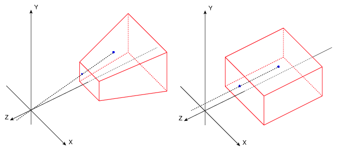
With a per­spec­tive cam­era, pro­jec­tion hap­pens from the world, to­wards the “sensor,” which is a de­fined point. For the sake of ar­gu­ment, let’s say that point is at the ori­gin and the cam­era is fac­ing the pos­i­tive $z$ axis.

We want all other points to be pro­jected onto a plane $d$ dis­tance away. If you are a pho­tog­ra­pher, $d$ will be the fo­cal length of the cam­era.

Orthographic Projection

In the case of or­tho­graphic pro­jec­tion, this is easy. Be­cause we have placed the cam­era on the ori­gin, fac­ing the pos­i­tive $z$ axis, we can draw the co­or­di­nates of any given point di­rectly to the screen. The only con­sid­er­a­tion nec­es­sary per­tains to the points be­hind the cam­era, which we can skip by check­ing the sign of the $z$ com­po­nent.

Homogeneous Coordinates

This is where ho­mo­ge­neous co­or­di­nates come in. When work­ing in eu­clid­ean space, we rep­re­sent a given vec­tor or co­or­di­nate us­ing three com­po­nents:

$$\begin{bmatrix} x$$\\ y \\ z \end{bma­trix}

When we are work­ing in pro­jec­tive space, we can rep­re­sent any given vec­tor or co­or­di­nate us­ing four com­po­nents.

$$\begin{bmatrix} x$$\\ y \\ z \\ w \end{bma­trix}

We can con­vert be­tween these for­mats in­ter­change­ably. To con­vert a ho­moge­nous co­or­di­nate to eu­clid­ean, di­vide all other com­po­nents by $w$:

$$\text{euclidean co­or­di­nate} = \begin{bmatrix} x / w$$\\ y / w \\ z / w \end{bma­trix}

We can trans­form any eu­clid­ean co­or­di­nate to a ho­moge­nous co­or­di­nate by set­ting $w = 1$

$$\text{homogenous co­or­di­nate} = \begin{bmatrix} x$$\\ y \\ z \\ 1 \end{bmatrix}

Just like we can per­form var­i­ous trans­for­ma­tions on eu­clid­ean co­or­di­nates, we can per­form sim­i­lar ones on ho­moge­nous co­or­di­nates. The ma­jor dif­fer­ence: in­stead of re­quir­ing con­ven­tional ad­di­tions or sub­trac­tions, ho­moge­nous co­or­di­nates can be trans­lated via ma­trix mul­ti­pli­ca­tion.

For ex­am­ple, let’s say we have a point at the ori­gin, and we want to per­form both a trans­la­tion and ro­ta­tion. If we were us­ing eu­clid­ean co­or­di­nates, we would have to trans­late it via ad­di­tion, then ro­tate it sep­a­rately.

$$\begin{bmatrix} 0 & 1 & 0$$\\ -1 & 0 & 0 \\ 0 & 0 & 1 \\ \end{bmatrix} \left( \begin{bmatrix} 0 \\ 0 \\ 0 \end{bmatrix} + \begin{bmatrix} 1 \\ 2 \\ 0 \end{bmatrix} \right) = \begin{bmatrix} 2 \\ -1 \\ 0 \end{bmatrix}

In ho­moge­nous co­or­di­nates, we can do it with a sin­gle ma­trix op­er­a­tion by prepar­ing the ma­trix ahead of time:

$$T = \begin{bmatrix} 0 & 1 & 0 & 0$$\\ -1 & 0 & 0 & 0 \\ 0 & 0 & 1 & 0 \\ 0 & 0 & 0 & 1 \end{bmatrix} \begin{bmatrix} 1 & 0 & 0 & 1 \\ 0 & 1 & 0 & 2 \\ 0 & 0 & 1 & 0 \\ 0 & 0 & 0 & 1 \end{bmatrix} $$T \begin{bmatrix} 0$$\\ 0 \\ 0 \\ 1 \end{bmatrix} = \begin{bmatrix} 2 \\ -1 \\ 0 \\ 1 \end{bmatrix}

By con­dens­ing the en­tire trans­for­ma­tion into a sin­gle ma­trix, we are able to save a ton of com­put­ing time.

Perspective Projection

The es­sen­tial idea of per­spec­tive pro­jec­tion is sim­ple: we want points fur­ther from the cam­era to ap­pear closer to the $z$ axis the fur­ther away they are. Re­mem­ber that $d$ is the sur­face we are pro­ject­ing onto. This is pos­si­ble with ho­moge­nous co­or­di­nates with the fol­low­ing ma­trix:

$$\text{perspective pro­jec­tion ma­trix} = \begin{bmatrix} 1 & 0 & 0 & 0$$\\ 0 & 1 & 0 & 0 \\ 0 & 0 & 1 & 0 \\ 0 & 0 & -1 / d & 1 \end{bmatrix}

Assuming you have an un­der­stand­ing of ma­trix mul­ti­pli­ca­tion, it should be ap­par­ent why this works. When the $w$ com­po­nent of the ma­trix is be­ing com­puted, the $z$ com­po­nent will be di­vided by $d$. The re­sult then be­comes a di­vi­sor of $w$, which af­fects all com­po­nents of the re­sult­ing vec­tor due to the na­ture of ho­moge­nous co­or­di­nates. In short: $w \leftarrow w * (-z / d)$

Color

Now that we’ve es­tab­lished ex­actly how to pro­ject points in space onto the screen, we need to start col­or­ing in tri­an­gles. As I said be­fore, I am not go­ing to go into the al­go­rithms that do this. I want to dis­cuss how to de­ter­mine the color to fill in.

We could just choose one solid color. As you can see from the demo (by press­ing R), this does­n’t lead to a par­tic­u­larly im­pres­sive or vi­su­ally pleas­ing re­sult. I want an ad­di­tional way to con­vey depth.

Given the three points that make up a tri­an­gle $p_1$, $p_2$, and $p_3$, we can find its nor­mal vec­tor (the vec­tor per­pen­dic­u­lar to it’s sur­face), $\vec{n}$ fairly eas­ily.

$$\vec{h} = \frac{p_2 - p_1}{||p_2 - p_1||} \times \frac{p_3 - p_1}{||p_3 - p_1||}$$ $$\vec{n} = \frac{h}{||h||}$$

Note: the ver­ti­cal bars around a vec­tor $||\vec{v}||$ sig­nify get­ting the vec­tor’s length.

Now that we have the tri­an­gles nor­mal, we can fill it in more brightly de­pend­ing on how di­rectly it is fac­ing the cam­era.

$$\text{brightness} = \vec{n} \cdot ||\frac{p_1 + p_2 + p_3}{3}||$$

The re­sult­ing shad­ing is the de­fault in the demo.

Alternatively, we can also sim­ply color based on the dis­tance from the cam­era. The re­sult­ing im­age is called a depth map.

$$\text{brightness} = \text{view dis­tance} - ||\frac{p_1 + p_2 + p_3}{3}||$$

Sorting

When the pro­gram is sup­plied a mesh, the faces are not in any spe­cific or­der. If we were to just draw each face in the or­der it ar­rives, noth­ing would make sense.

To solve this, we sim­ple sort each face by it’s dis­tance, then draw the fur­thest faces first.

If you want to see what it would look like, go to the demo and press O to tog­gle face sort­ing.

Optimization

There are count­less ways to op­ti­mize a ren­derer like this. They all in­volve work-avoid­ance. The one I want to dis­cuss is of­ten re­ferred to as back­face culling.

In most sit­u­a­tions, there is no need to see the in­side of a mesh. This al­lows us to avoid a lot of work for very lit­tle ef­fort. By check­ing the align­ment of the point-to-face vec­tor with a face’s nor­mal, we can check if a given face is fac­ing to­ward us or not.

In the demo, you can tog­gle back­face culling with B.

Conclusion

When I ini­tially de­signed this pro­ject, I hoped it would al­low me to ap­ply some of the more ad­vanced lin­ear al­ge­bra con­cepts that I’ve learnt in the sec­ond trimester. In this re­gard, it did not live up to my ex­pec­ta­tions.

While I was al­lowed to ex­plore some con­cepts, like or­thog­o­nal­ity, it was not quite sat­is­fac­tory.

It was not for naught, though. I learned a lot about the fields of math and com­put­ers in­te­grate to­gether, as well as how to more ef­fec­tively con­vert math­e­mat­i­cal con­cepts into a work­ing pro­to­type. I want to con­tinue do­ing pro­jects like this, and can­not wait to re-take Linear Algebra when I go to col­lege.